How to know when machine learning does not know
by Nicolas Papernot and Nicholas Frosst
It is becoming increasingly important to understand how a prediction made by a Machine Learning model is informed by its training data. This post will outline an approach we call Deep k-Nearest Neighbors [Papernot and McDaniel] that attempts to address this issue. We will also explore a loss function we recently introduced to shine some light on how models structure their internal representations [Frosst et al.]. We’ll illustrate how the Deep k-Nearest Neighbors (DkNN) helps recognize data that is not from the training distribution by observing anomalies in the internal representation of such data.
Consider adversarial examples. Constructing an adversarial example does not require any modification to the model’s training data. Yet, being able to tie the model’s prediction back to some of its training points could still help distinguish adversarial examples from legitimate test inputs. Imagine that the nearest training points in hidden layers have a very different label than what is predicted on a test example. This could be an indicator that the test example has been adversarially manipulated.
This is what we illustrate next. Here’s a test input. Use the slider below it to turn the input into an adversarial example (moving the slider to the right will make the input increasingly more adversarial).
As you move the slider, you can visualize below how the input is being embedded by the different layers of the neural network. Originally, when the slider is fully to the left, the input is close to training points from its own class (the label of training points is shown when hovering over them). As you move the slider to the right to make the input increasingly adversarial, the input will get increasingly close from points in a wrong class. This will first happen at layer 3 (the output layer), then layer 2, and finally layer 1.
If you’d like to retrain the model from scratch, you can do so using this button:
This type of analysis could also be useful to detect attempts at poisoning the model’s training data: an adversary may intentionally introduce errors in the training data to poison our model. If we are able to identify the training points that led to an incorect model prediction, it is likely that among these training points we’ll find the ones manipulated by the adversary. We could remove them and retrain the model without the poison.
Why is estimating support from the training data important?
Even in cases where adversaries are not a concern, establishing a notion of support from the training data could strengthen the usability of systems that integrate machine learning. This often proves to be important when safety is at stake. Take the example of a medical practicioner analyzing the diagnosis made by a ML system. Knowing which training medical records the model draws from when making a diagnosis on a new patient would help the practicioner avoid either blindly trusting the model or not trusting the model at all, both extrema being undesirable to patients.
More generally, as the ML community moves towards an end-to-end approach to learning, models are taking up roles that used to be fulfilled by pre-processing pipelines. Features are no longer manually engineered to extract a representation of the input. A good example of that is machine translation—significant progress was made by replacing systems engineered for several decades with a holistic sequence-to-sequence model. This lack of pre-processing pipeline generally means that the input domain is less constrained. Despite this, models are deployed with little input validation, which implicitly boils down to expecting the classifier to correctly classify any input that can be represented by their input layer. This goes against one of the fundamental assumptions of machine learning: models should be presented at test time with inputs that fall on their training manifold. Hence, if we deploy a model in an environment were inputs may fall outside of this data manifold, we need mechanisms for figuring out whether a specific input/output pair is acceptable for a given ML model. In security, we sometimes refer to this as admission control. This is what we’d like to achieve by estimating the training data support for a particular prediction.
Before we dive in the details of how exactly we can do that, let’s take a step back and outline some of the things we could do once we are able to identify training points that support a classifier’s prediction:
-
uncertainty: when a prediction is supported by training points from different classes of the data, we can infer that the test point we are trying to classify is ambiguous. In other words, the test point presents characteristics of training points from multiple classes and the classifier should not classify it with confidence in any single class. This uncertainty comes from the fact that the classifier learned from limited data. It is also sometimes called epistemic uncertainty.
-
outlier detection: in cases where we are able to detect ambiguity and measure high uncertainty in the prediction being made by the classifier, we could refuse to reveal the classifier’s prediction. This boils down to detecting out-of-distribution examples. These test inputs may not be on the training manifold because they were manipulated by adversaries or simply because they represent a legitimate situation we had not foreseen during training.
-
active learning: if we are able to identify when the classifier is making a prediction not well supported by the training data and we know that this is an important prediction, then we can have more training data collected and labeled in this region of the input domain to help increase the support of our model for this type of predictions.
-
interpretability: in domains such as vision where the training points and labels are easily interpreted by humans, training points that make up the support for a prediction may provide valuable insights into some of the correlations used by the model to classify a given test input.
So how does the DkNN help?
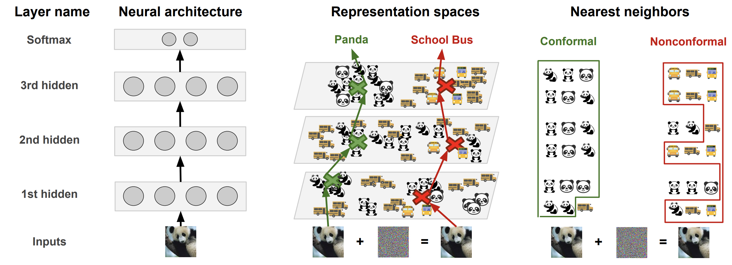
The DkNN can be thought of as a hybrid classifier that takes in an existing deep neural network (a DNN) and uses its internal representations to perform a k-nearest neighbors (kNN) search. Hence the name Deep k-Nearest Neighbors (DkNN). Let’s see how this works in practice.
When a normal DNN classifies an input, the input is transformed by a succession of layers. Each layer analyzes its inputs looking for certain patterns among the features extracted so far and outputs a new representation of the input. Eventually, as we reach the last layer of the model architecture, the representation is sufficiently abstract to compute a score for each class. These scores are called the logits. The label predicted by the model is simply the class that has the largest logit.
In addition to a prediction, DNNs also output a confidence value. This value is computed by a softmax, which takes the scores assigned to each class and normalizes them to produce a vector of values that sum up to 1 across all classes. Despite being often referred to as softmax probabilities, these values are not reliable estimates of the model’s confidence. One demonstration of this is that they can be gamed: an adversary can often arbitrarily control with how much confidence a neural network equiped with a softmax will misclassify the adversarial example.
To avoid these pitfalls, the Deep k-Nearest Neighbors (DkNN) breaks the black-box myth around deep learning. It harnesses the intrinsic modularity of deep neural networks: they are made up of a stack of layers. Patterns extracted by hidden layers on a test input are compared to those found during training to ensure that when a label is predicted, patterns that led to this prediction can be found in the training data for this label. By doing that, we are able to measure uncertainty in a way different from how neural networks typically compute class scores. When a prediction at test time is the result of model behavior that is not conformal with model behavior observed on the training data, this indicates the model is largely speculating. Such a prediction is uncertain and should not be trusted.
Finding nearest neighbors
Assume we are given a point x that we’d like to classify with the DkNN.
We first need a way to compare the behavior of the neural network on this test
point with the behavior of the neural network on its training data.
To make this comparison easier, we leverage the modularity provided by the model’s
layers. Indeed, the output of each layer can be though of as a snapshot of
the logic followed by the neural network to analyze the input and extract
more and more abstract information from it—until the model is able to predict
the class the input belongs to.
We first run the point x through the neural network and record the output of each
layer on the test input. Our goal is then
to identify, for each layer, k points in the model’s training set for which the layer
outputs representations that are most similar to the test point’s representation.
We do this through a k-nearest neighbor search on the output of the layer when it is presented with training points. It returns the k training
points whose representations are most similar to the representation of our
test point. By repeating this process for each layer, we obtain a set omega(x) of L * k neighbors
for point x where L is the number of layers in our model and k is the
number of neighbors found at each layer.
Estimating uncertainty with conformal prediction
Because the L * k neighbors from omega(x) are from the training set, we have labels for
each of these points. The DkNN uses the homogeneity of these labels as a proxy
for the model’s (un)certainty in predicting a label. If all of the nearest
training points have the same label across all layers and the model predicts
that same label, the (input, prediction) pair is conformal with the training data and
the prediction has high certainty. On the other hand, if the
labels indicate that the nearest training points come from many different classes,
the prediction has high uncertainty.
To set an expectation on the level of homogeneity needed for a prediction to be
certain, we apply the framework of conformal prediction. In particular, we
consider a holdout set of labeled data, the calibration dataset, that is neither
used to train nor test the model. For each of the calibration points (x, y) ,
we compute the nonconformity alpha(x, y) of the point x for label y defined as
the number of training neighbors in omega whose label is different from y.
When classifying a test input x, we then follow these steps:
-
Find the set
omega(x)of neighboring training points by performing a nearest neighbor search in each of theLlayers of the model. -
For each class
jof the task, compute the nonconformityalpha(x, j)of classifyingxin classj: this nonconformity is the number of neighboring training points inomega(x)whose label differs fromj. -
Compute the ratio between (a) the number of calibration points whose nonconformity is larger than the nonconformity of the test point and (b) the total number of calibration points. This ratio is the empirical p-value associated with class
jfor inputx. -
Predict the label
jwhose empirical p-value is largest. This DkNN prediction comes with an estimate of its uncertainty called the credibility. Credibility is defined to be the empirical p-value of the prediction made.
By following this procedure for each input, the DkNN makes predictions that potentially differ from predictions made by the original neural network whose representations are used to find neighboring training points. This typically happens when the original neural network’s prediction was wrong or uncertain. Instead, DkNN predictions come with a credibility value, which can serve as the basis for building mechanisms that reject such inputs for which uncertainty is too high.
Detecting out-of-distribution inputs with credibility
To see how credibility helps identifying inputs that are not part of the distribution a neural network was trained to model, let us take the example of a model trained on one dataset but tested using the validation set of a different dataset. Here, we’ll consider two pairs of datasets:
-
a neural network trained on MNIST (a dataset for handwriting recognition) and tested on NotMNIST (a dataset of characters rendered using computer fonts). While both datasets share the same input dimensionality (28x28 grayscale images), their classes are non-overlapping: MNIST classes are digits between 0 and 9 while NotMNIST classes correspond to letters between A and J. Thus, we don’t expect a network trained on MNIST to perform well when presented with NotMNIST images.
-
a neural network trained on SVHN (a dataset for digit recognition) and tested on CIFAR10 (a dataset for object recognition). Here again, both datasets have the same input dimensionality (32x32x3 color images) but non-overlapping classes: we don’t expect a model trained on one dataset to perform well on the other.
For each of the two datasets, we train a neural network on the first (respectively MNIST and SVHN) and use the same model to make predictions on the second (respectively NotMNIST and CIFAR10). We also record the confidence values output by the softmax of the neural network for each prediction. We then repeat the experiment, this time predicting with the DkNN and reporting the credibilty of each prediction.
In the Figure below, we group test points according to their softmax confidence
or DkNN credibility into bins of size 0.1. Because both uncertainty estimates range between 0 and 1,
test points are split across 10 bins. We expect all test points to be assigned low confidence and credibility
because they are not part of the distribution the two models were trained on.
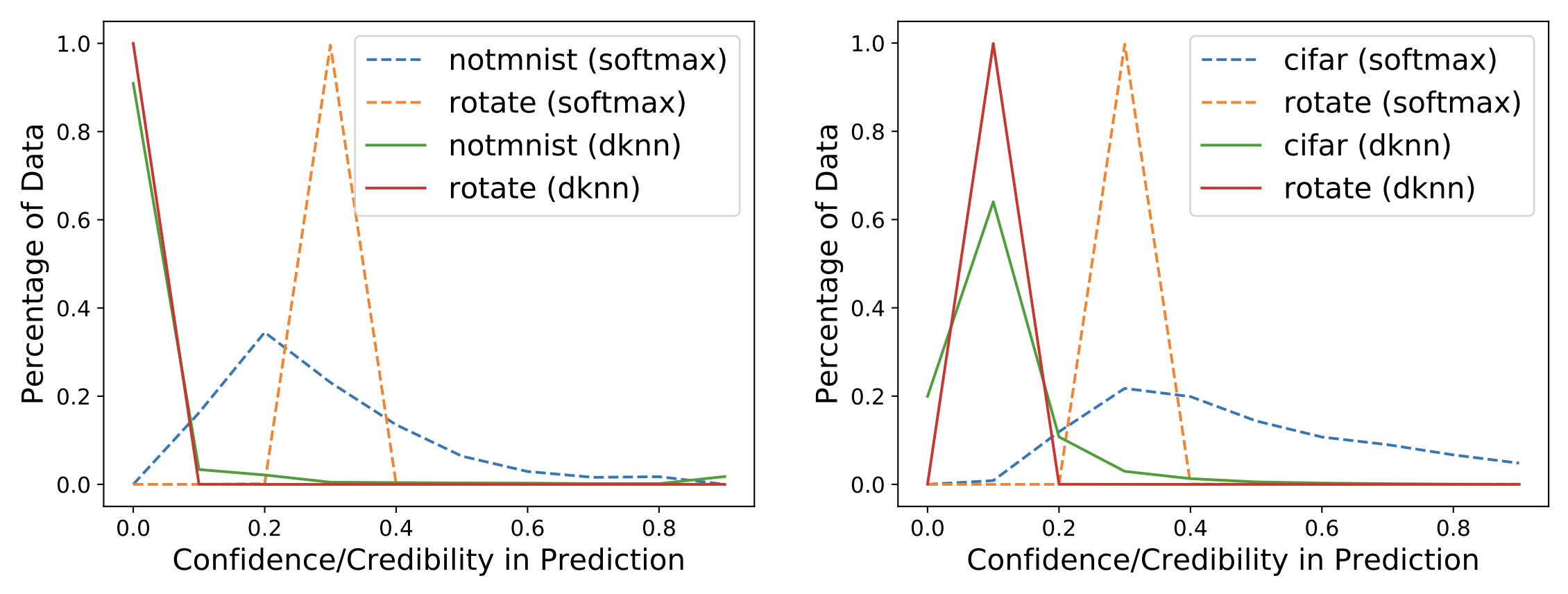
This is not exactly what happens: as shown on the left, the MNIST model outputs medium to high confidence, according to its softmax, on a large part of the NotMNIST test set (see blue dotted line). This is not desirable: the model was not trained to classify these inputs so it should have low confidence. Instead, the DkNN, which relies on the same underlying neural network, outputs low credibility on all NotMNIST test points (see green solid line). The DkNN is able to capture more accurately high prediction uncertainty that results from the lack of support from training data—as the neural network infers on out-of-distribution inputs. The Figure on the right shows similar results when comparing the softmax confidence and DkNN credibility of a neural network trained on SVHN and tested on CIFAR10: softmax confidence is fairly high for a large portion of the CIFAR10 test set (see blue dotted line) whereas DkNN credibility is consistently low across the entire test set (see green solid line).
Both Figures also contain an additional experiment where the model is presented with images from the correct test set which have been rotated to simulate a different outlier test distribution. Again the DkNN credibility (red solid lines) is consistently lower than the softmax confidence (orange dotted lines), reflecting epistemic uncertainty that underlies the model’s predictions.
Characterizing uncertainty when predicting on adversarial examples with the DkNN
Now that we demonstrated how the credibility output by the DkNN along with each prediction improves how we can distinguish legitimate inputs from out-of-distribution inputs by better capturing uncertainty, it is natural to wonder whether this behavior can also be obtained on worst-case test inputs like adversarial examples.
Here again, we compare how uncertainty is estimated by the neural network’s softmax and the DkNN credibility. The following graphs illustrate how the two uncertainty estimates compare on a traffic sign classification dataset called GTSRB where the test data was modified with the BIM attack. This attack is also known as PGD (the only difference introduced by PGD over BIM is a random restart step before the gradient descent). The DkNN paper contains similar results on MNIST and SVHN, as well as with other attacks like the Carlini and Wagner attack.
Each plot is generated by grouping test points into bins corresponding to the softmax confidence or DkNN credibility of their prediction. There are 10 bins dividing the range of possible confidence/credibility values between 0 and 1. The red curve visualizes the density of data in each bin: that is, the number of test points that were asssigned the confidence or credibility corresponding to this bin. In addition, each blue bar indicates the average accuracy of predictions made within the corresponding bin.
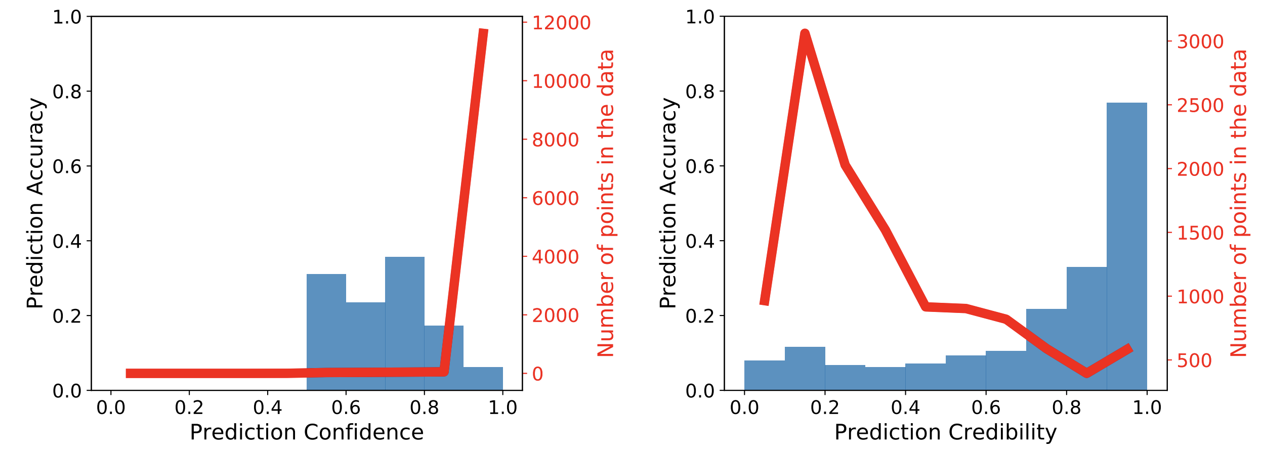
On the left, we observe that the softmax confidence is high on most adversarial
examples because the red curve shows that most points fall in the bin corresponding
to a confidence larger than 0.9. The blue bar for this bin is quite low, reflecting
the fact that the neural network is making incorrect predictions despite having high
confidence in these predictions. The adversary was successful here.
Instead, on the right, the DkNN credibility assigns
mostly low credibility scores to adversarial examples because the red curve peaks
for credibility bins around 0.2. The DkNN identifies an inconsistency
between the model’s internal representations on adversarial examples and their nearest
neighbors in the training data, which explains why they are assigned low credibility.
The DkNN is even able to recover the correct label for a small subset of these adversarial
examples because the labels of the nearest training points still largely agree
on the correct label. This is shown by the high blue accuracy bar for the
bin corresponding to a credibility larger than 0.9
We are not claiming here that the underlying model is now robust to adversarial examples. The neural network is in fact unchanged. Instead, we argue that an inference procedure that departs from simply outputting softmax predictions may help to distinguish legitimate test inputs from out-of-distribution inputs such as adversarial examples or test inputs from a different dataset. The DkNN enables this distinction by improving how uncertainty is captured and introducing the credibilty metric. It remains an open problem to fully explore the space of possible inference procedures that build on architectures trained with current learning algorithms.
Adaptive attacks against the DkNN
To conclude our evaluation, we consider ways that an adversary could adapt to the credibility metric and try to game it. The adversary’s goal is to find adversarial examples for which the DkNN outputs high credibility in the wrong class. This would be an effective attack because it would make it difficult for the defender to set a threshold on credibility that is large enough for detecting outlier inputs (e.g, out-of-distribution or adversarial examples) but low enough to limit the number of legitimate test inputs that are flagged as outliers.
Intuitively, a successful attack would produce an adversarial example whose neighboring training points are labeled in the wrong class (the class that the adversary is trying to have the model predict). We know that intermediate hidden representations can be manipulated with an attack called feature adversaries [Sabour et al.]. To attack a source image, the adversary chooses a guide input and modifies the source image to push the neural network towards predicting a hidden representation on the modified image that is more similar to the one it infers on the guide image. Sabour et al. demonstrated the attack on hidden layers that are located towards the middle or output of the model architecture.
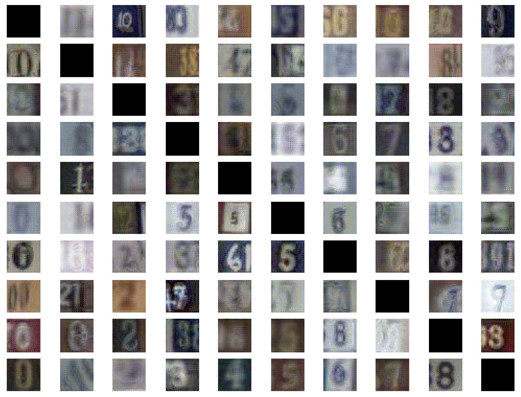
In order to adapt this attack to the DkNN, we need to (a) find good guide images and (b) modify enough of the internal representations for the credibility metric to be high on the modified image. The DkNN paper proposes to address (b) by targeting the first hidden layer: once the input has a representation close to a wrong class at the first hidden layer, representations through the remainder of the model architecture will also be consistent with that wrong class. Hence, credibility will be high on that input. The training image whose representation in the target class is closest to the representation of the input being attacked is selected as the guide image. This mounts a targeted attack: the adversary chooses the wrong class predicted by the DkNN.
The following matrix plots some of the adversarial examples produced by this attack on SVHN. Images are organized such that their row index indicates the source class of the image and their column index corresponds to the target class. All inputs are classified by the DkNN in the target class, however many of these inputs are ambiguous. The attack modified input semantics in order to evade the DkNN.
[Sitawarin and Wagner] recently improved upon this attack strategy, albeit in the untargeted setting, by having the adversary optimize an attack objective that involves a differentiable approximation of the k nearest neighbors. While they claim in their introduction and Section VII.B that their attack can find adversarial examples for the DkNN, we reiterate that an adversary needs to consider the credibility metric to ensure that adversarial examples are assigned high credibility. As such the evaluation performed in Section VII.B of their paper is not sufficient to draw conclusions on the robustness of the DkNN. In fact, the authors acknowledge later in Section VIII that adversarial examples are assigned low credibility (see Figure 5). This low credibility may be a consequence of the untargeted nature of the attack: the class of guide images is chosen to be the class closest in representation space to the input being attacked, which makes it easier to attack the DkNN, but also results in ambiguous adversarial examples (e.g., 3s turned into 8s by completing loops in Fig 1 or 6s faded out to 5s in Fig 3).
Adversarial examples typically gradually turn a small change in the input domain into a large change in the model’s output space. This results in layers closer to the input of the model having representations that are closer to the correct class of the input while layers towards the output having representations that are closer to the wrong class. Credibility helps distinguish legitimate data from outlier data by forcing inputs to have the same degree of consistency than calibration data across the network’s architecture.
Improving the similarity structure of representations
All of the results we described so far applied the DkNN to a deep neural network without making any changes to how it is trained. A simple strategy for improving how representations handle known outliers would be to adversarially train the neural network. We chose not to explore this direction because it forces the defender to react to known attack strategies. Similarly, most data augmentation techniques are specific to a particular set of tasks: e.g., vision tasks.
Instead, we modify the training objective of our neural network to improve the similarity structure of its hidden representations analyzed by the DkNN. The similarity structure of data representations is a vast topic. Here, we are primarily interested in how close pairs of representations from the same class are relative to pairs of representations from different classes. This is sometimes referred to as entanglement. If we have very low entanglement, then every representation is closer to representations in the same class than it is to representations in different classes.
In a recent paper to appear at ICML 2019, we explored the soft nearest-neighbor loss as a tool to track the evolution of entanglement during learning [Frosst et al.]. This led us to a surprising observation: encouraging representations to entangle data—that is to bring points from different classes closer together—improved the similarity search performed by the DkNN more than encouraging representations to disentangle data—which would help achieve a large margin between classes like SVMs.
One possible explanation for this is that by encouraging the model to entangle hidden representations while discriminating between classes at the logits layer, we possibly encourage representations to identify class-independent similarity structures. Our hypothesis is that this would in turn mean that the nearest neighbor search performs better:
-
in ambiguous regions of the input domain between dense clusters of points, because entangled representations force these different class clusters to spread out and overlap more in these ambiguous regions.
-
on outlier inputs, which are projected further away from the training manifold, because their representations do not share any of the features specific to a class or co-adapted between classes.
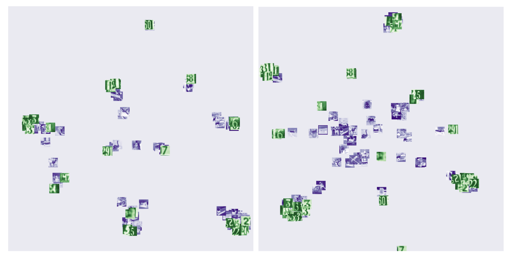
We illustrate the behavior described in the second bullet point with the following Figure. It is a 2D visualization of the logits of a model trained with cross-entropy only (left) and a model trained with both cross-entropy and the soft nearest-neighbor loss to simultaneously discriminate classes and entangle data (right). Points in green are in-distribution, this is a SVHN model. Points in blue are out-of-distribution, they are from the CIFAR10 test set. The out of distribution data is easier to separate from the true data for the entangled model than it is for the baseline model.
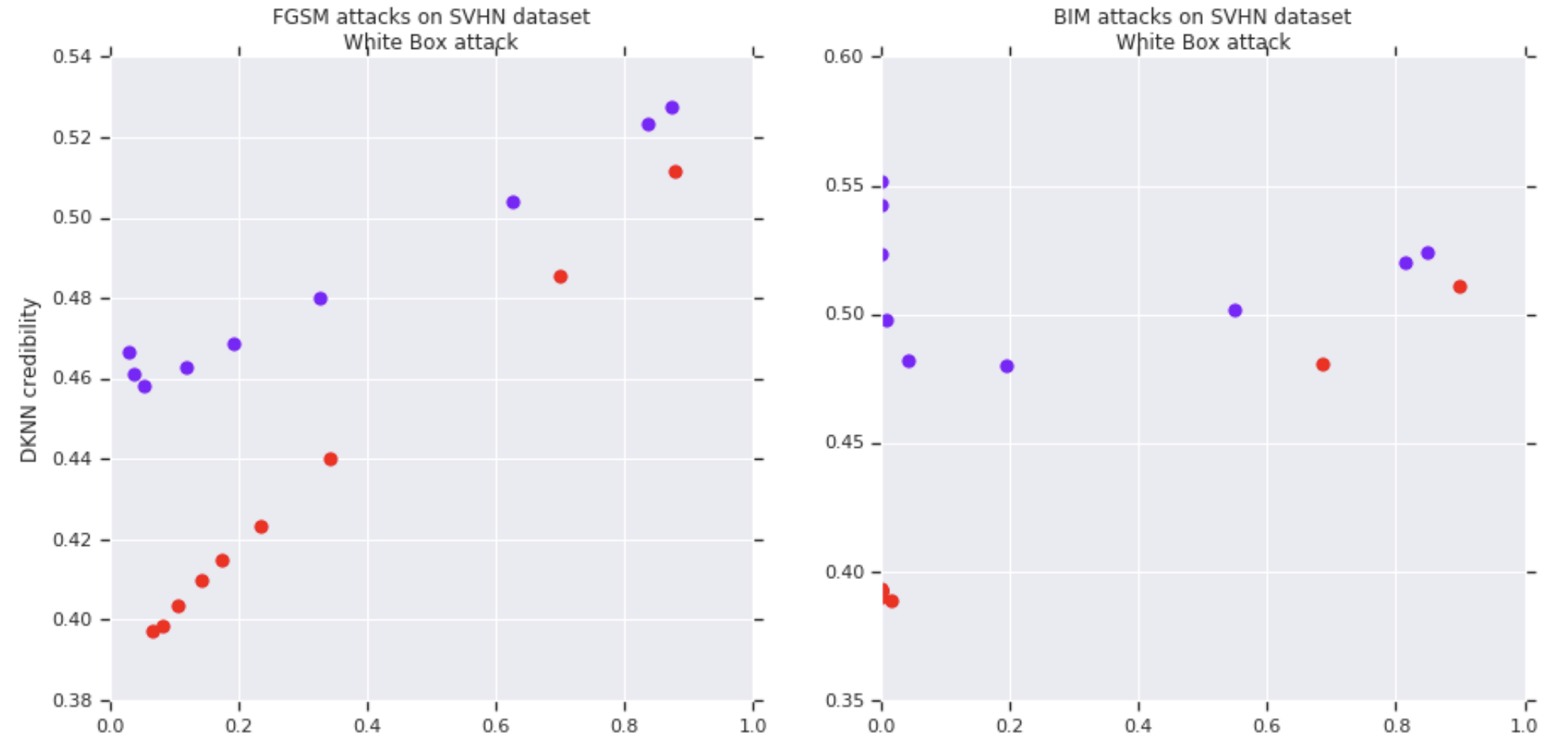
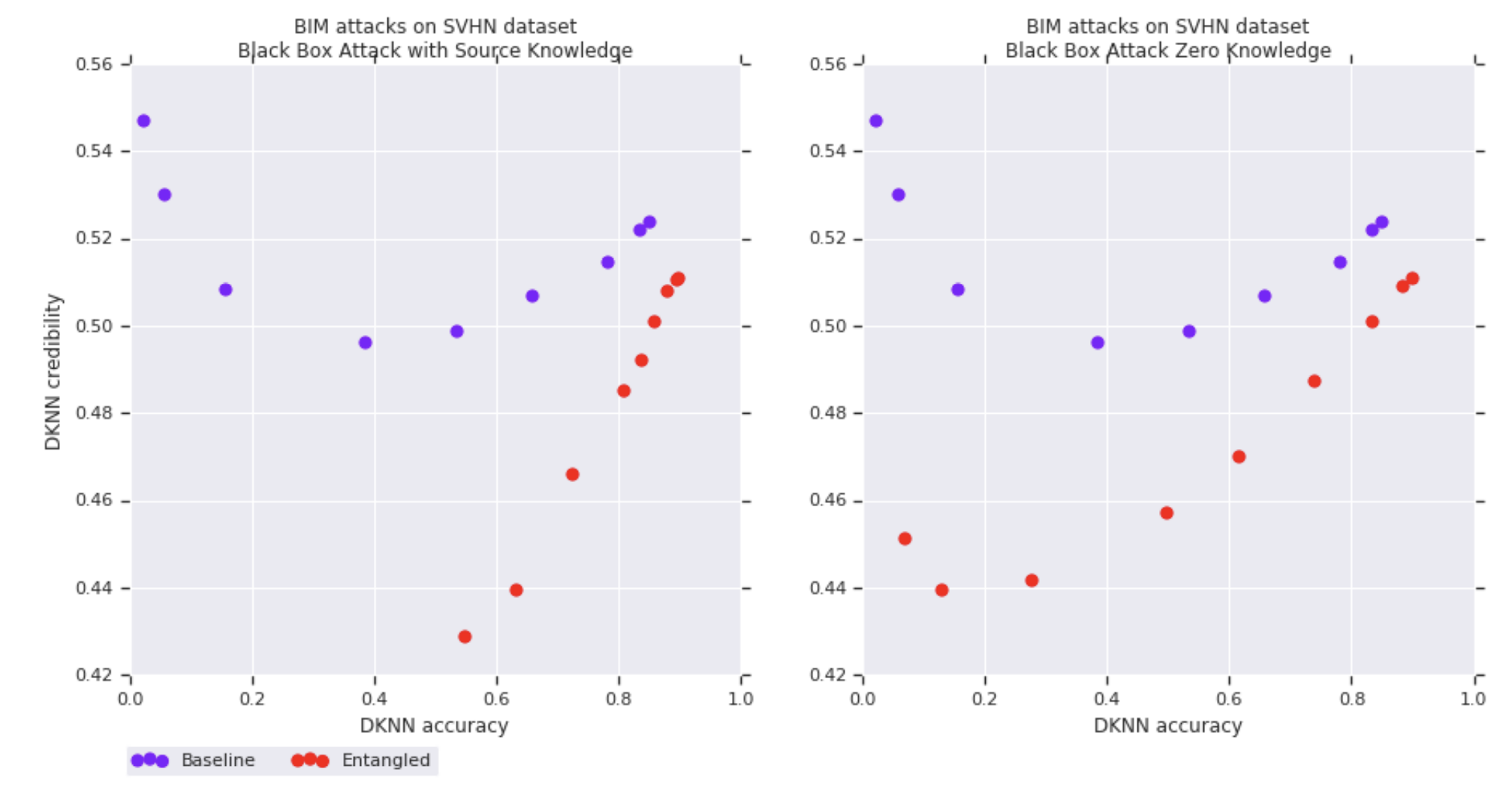
Entangled models also improve the correlation between credibility estimates and prediction accuracy on adversarial examples. The following figures show on the vertical axis the DkNN credibility and on the horizontal axis the DkNN prediction accuracy. Each curve is plotted by varying the attack strength on a baseline (purple) or entangled (red) SVHN model. Each of the 4 figures corresponds to a different attack: white-box FGSM (top left), white-box BIM (top right), black-box from entangled model (bottom left), black-box from baseline model (bottom right).
Results on other datasets, as well as implications of the soft nearest-neighbor loss for other ML tasks such as generative modeling, are discussed in the paper.
Conclusions
Perhaps the most interesting aspect of our work is to show that there exist interesting alternatives to simply outputing softmax predictions at test time. In our work, we analyze the similarity structure of hidden representations to estimate the uncertainty of predictions and recognize data that is not from the training distribution. We hope this will inspire others to pursue this research direction.
Acknowledgements
We’d like to thank David Berthelot for comments on a draft of this document. We also thank the authors of TensorFlow.js and the JS implementation of UMAP.